
Written by: Thomas van Osch
Aerodynamics of a F1 car, the stock price of Tesla, the spread of diseases and the simulation of black holes – what do these concepts have in common?
These are just some examples where (partial) differential equations can help model and understand phenomena that would be otherwise difficult or even impossible to explain. Instead, partial differential equations give a wide variety of domains a mathematical framework to describe very complex systems. As you can imagine, solving these powerful equations is not a trivial task. So how do we approach this and where does HPC come into play?
Too ordinary?
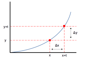
Let’s first get comfortable with differential equations. The term differential describes how one quantity changes with respect to another quantity. See the graph below with two axes. On the horizontal axis we measure some quantity with x against some quantity of y on the vertical axis. The relationship between these two quantities is depicted by the blue line as a function. Assume now we want to model the speed (y-axis) of a car over time (x-axis).
From the blue line we can see the car first needs to start its engine and reach a good acceleration before the speed goes up fast. By using derivatives, we can find within a timespan Δx between x and x + t, say between 1 minute and 2 minutes, how much the car has accelerated in terms of Δy. Or more technically, the derivative describes the rate of change in speed. This is very us
eful as it provides insight into how different phases of the acceleration of the car behave. From here, we can see where the acceleration can be improved and compare the speed to other cars.
An Ordinary differential equation
Solving a differential equation means finding the function that satisfies the equation. In our car example, the single variable of speed can be described in a single function to model the speed over time. Equations where an individual variable changes with respect to a single other variable is called an ordinary differential equation. In the real world, the function may not always be ordinary and multiple variables influence what we want to measure. So how do we approach this?
How to understand: an example of partial differentials in action
Imagine you are trying to predict the movement of water in a river. The speed and direction of the current is measurable at each point in the river. However, we want to know how the current will change in the future (time) and at various locations (space). Another difficulty is that we need to keep in mind the different factors such as the water flow rate, the shape of the riverbed, the friction of the ground, etc. All these variables impact the current. With partial differentials, we can derive the function of the water current and the impact of the individual factors. PDEs then give us a framework to model the relationship between individual variables to a certain quantity over time and space.
Often in complex physical systems with many interacting variables and factors, the mathematical function to model the physical phenomenon is difficult to accurately solve. Even then, these solutions may not be stable or reproducible. We usually need to solve PDEs by taking small steps to get closer and closer to the true solution. Even each of these small steps involve a large amount of computations. Here is where computers come into play, as we will see below.
So, while partial differential equations might sound complicated, in essence they are just a tool that scientists use to understand how things move and change in the world around us.
Scaling Partial Differential Equations (PDEs)
Computations to derive a solution for PDEs are costly and time-consuming. In practice, PDEs often involve performing operations on large matrices in which high-performance computing shines. By decomposing the matrices, enabling large-scale parallel processing and developing HPC-specific numerical methods, accurately approximating these PDEs become more feasible. On top, applying deep learning on partial differential equations and the increasing prominence of GPU infrastructure in computing clusters open up even more possibilities.
As researchers continue to develop new technologies and numerical methods to better approximate partial differential equations, while the community keeps on building larger and more data centers, the combination of PDEs and HPC has already led and will continue to lead us to significant breakthroughs in our understanding of physics, economics and social sciences – just to name a few of the vast landscape where PDEs can make a difference. Who knows what PDEs will tell us about the origin and future of our universe?
SURF
From the perspective of SURF, a national competence center, we have seen a rise in consultancy requests and cutting-edge research on partial differential equations coming from different domains. In specific, deep learning is now being combined with PDEs to arrive at more accurate solutions and predictions on weather forecasting, molecular structuring and more. The machine learning team within SURF is also developing generic neural PDE solvers to understand the concept and offer not only HPC infrastructure, but also technical and scientific insights in further improving these models.